Pathfinding Demystified (Part I): Generic Search Algorithm

Introduction

Pathfinding is one of these topics that usualy baffles game developers. The A* algorithm in particular is poorly understood, and the general belief seems to be that it’s arcane magic.

The objective of this series of articles is to explain pathfinding in general and A* in particular in a very clear and accessible way, and put an end to the misconception that it’s a difficult topic. Properly explained, it’s quite straightforward.

Note that the focus is on pathfinding for games; unlike a more academic approach, we’ll just skip search algorithms such as Depth-First or Breadth-First. Instead, we’ll try to go from zero to A* as quickly as possible.

This first article explains the very basic concepts of pathfinding. Once you get these basic concepts, you will find A* surprisingly simple.

A Simple Setup

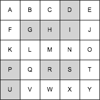
Although you’ll be able to apply these concepts to arbitrarily complex 3D environments, let’s start with an extremely simple setup: a 5 x 5 square grid. For convenience, I’ve labelled each square with an uppercase letter.

The very first thing we do is to represent this environment as a graph. I won’t go into the details of what a graph is; intuitively, it’s a set of bubbles connected by arrows. The bubbles are called “nodes”, and the arrows are called “edges”.

Each node represents a “state” your character can be in. In this case, the state of your character is its position, so we create one node for each square of the grid:

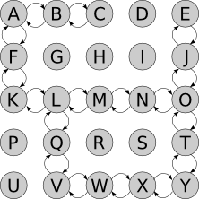
Now let’s add the edges. These represent what states you can “reach” from any other given state; in this case, you can walk from any square to an adjacent square, except for the blocked ones:

If you can get from A to B, we say B is “adjacent” to A.

Note that edges are directional; we need both an edge from A to B and an edge from B to A. This may look redundant, but it isn’t when you consider more complex “states”. For example, you can fall from the roof to the floor, but you can’t jump from the floor to the roof. You can move from “alive” to “dead”, but not the other way around. And so on.

An Example

Say we want to go from A to T. We start at A. We can do one of exactly two things: walk to B, or walk to F.

Suppose we walk to B. Now we can do two things: go back to A, or walk to C. We remember we’ve been in A already, and we’ve considered our options there, so it’s pointless to do it again (otherwise we could spend all day going A → B → A → B…). So we go to C.

Now at C we have nowhere to go. Going back to B is pointless. So this is a dead end. Choosing B when we were at A wasn’t a good idea; maybe we should try F instead?

We just keep repeating this process until we find ourselves in T. At that point we just reconstruct the path from A, by retracing our steps. We’re at T; how did we get here? O? So the end of the path is O → T. How did we get to O? And so on.

Keep in mind that we didn’t actually move at all; all of this was a thought exercise. We’re still standing at A, and we won’t move at all until we have figured out the whole path. When I say “move to B”, I’m actually saying “imagine we moved to B”.

The General Algorithm

This section is the most important part of this whole series. This is the section you absolutely need to understand in order to do pathfinding; the rest (including A*) are mere details. This is the section where you achieve enlightenment once you get it.

This section is also embarrasingly simple.

Let’s try to formalize the example above into a bit of pseudocode.

We need to keep track of the nodes we know how to reach from the starting node. At the beginning this is just the starting node, but as we “explore” the grid we’ll figure out how to reach other nodes. Let’s call this list reachable:

reachable = [start_node]

We also need to keep track of the nodes we’ve already considered, so we don’t consider them again. Let’s call it explored:

explored = []

Here comes the core of the algorithm: at each step of the search, we choose one of the nodes we know how to reach but haven’t explored yet, and see what new nodes we can reach from there. If we find out we can reach the goal node, we’re done! Otherwise we keep looking.

Sounds disappointingly simple? It is. But that’s all there is to it. Let’s write it step by step in pseudocode.

We keep looking until we either reach the goal node (in which case we’ve just found a path from the start node to the goal node), or until we run out of nodes to look at (in which case there’s no path between the start node and the goal node).

while reachable is not empty:

We choose one of the nodes we know how to reach and haven’t explored yet:

node = choose_node(reachable)

If we’ve just figured out how to get to the goal node, we’re done! We just need to build the path, following the previous links back to the start node:

if node == goal_node:
   path = []
   while node != None:
        path.add(node)
        node = node.previous

    return path

There’s no point in considering a node more than once, so we keep track of that:

reachable.remove(node)
explored.add(node)

We figure out what nodes we can reach from here. We start with the list of nodes adjacent to this one and remove the ones we’ve already explored:

new_reachable = get_adjacent_nodes(node) - explored

We take each of these:

for adjacent in new_reachable:

If we already knew how to reach it, we ignore it. Otherwise we add it to the reachable list, keeping track of how we got there:

if adjacent not in reachable:
    adjacent.previous = node  # Remember how we got there.
    reachable.add(adjacent)

Finding the goal node is one way to exit the loop. The other one is when reachable becomes empty: if we run out of nodes to examine, and we haven’t reached the goal node at any point, it means there’s no path from the start node to the goal node:

return None

And… that’s it. Here’s the whole thing, with the code to build the path extracted into a separate method:

function find_path (start_node, end_node):
    reachable = [start_node]
    explored = []

    while reachable is not empty:
        # Choose some node we know how to reach.
        node = choose_node(reachable)

        # If we just got to the goal node, build and return the path.
        if node == goal_node:
            return build_path(goal_node)

        # Don't repeat ourselves.
        reachable.remove(node)
        explored.add(node)

        # Where can we get from here?
        new_reachable = get_adjacent_nodes(node) - explored
        for adjacent in new_reachable:
            if adjacent not in reachable
                adjacent.previous = node  # Remember how we got there.
                reachable.add(adjacent)

    # If we get here, no path was found :(
    return None

Here’s the function that builds the path following the previous links back to the start node:

function build_path (to_node):
    path = []
    while to_node != None:
        path.add(to_node)
        to_node = to_node.previous
    return path

That. Is. It. That is the pseudocode of every pathfinding algorithm, including A*.

Please re-read this section until you understand how it works, and perhaps more important, why it works. Doing an example by hand on a piece of paper would be perfect, but you can also try the demo below:

Live Demo

Here’s a live demo and a sample implementation of the algorithm above. choose_node just picks a node at random. You can run it step by step and see the list of reachable and explored nodes, and what the previous links point to.

reachable = [] explored = []

Note that the search stops as soon as a path is found; it may happen that some nodes are never even considered.

Conclusion

The algorithm presented above is the general algorithm for every pathfinding algorithm.

So… have you figured out what makes every algorithm different from each other - why A* is A*?

Here’s a hint: if you run the demo search above many times, you’ll see the algorithm doesn’t always find the same path. It finds some path, not necessarily the shortest path. Why?